Step one when dealing with automatic speech recognition systems is to identify features i.e. the audio signal elements we can actually use to identify crucial language content, while eliminating non-pertinent content such as white noise.

The main thing to understand about speech is the way human sounds are produced by the vocal tract manipulating sounds e.g. with the teeth, tongue etc. Specific shapes produce specific sounds.

Correctly identifying the shape should lead to an accurate prediction of the phoneme being spoken.

The vocal tract’s shape is embodied by the envelope of the short-time power spectrum, representing the envelope is – in fact – the function of MFCCs. In this guide, we will break down MFCCs.

Mel Frequency Cepstral Coefficient CA Guide 🇨🇦

---

Mel Frequency Cepstral Coefficients are a popular component used in speech recognition and automatic speech. They first came into play in the 1980s, designed by Davies and Mermelstein, and have since been the cutting edge standard.

Before MFCCs there were Linear Prediction Coefficients (LPCs) and Linear Prediction Cepstral Coefficients (LPCCs); the two features were used as main feature types for automatic speech recognition (ASR), in particular with HMM classifiers.

This tutorial will cover the crucial components of MFCCs, why they work well for ASR, and how to install them.

Brief Tutorial Overview

---

Let us begin with an eagle-eyed perspective introduction to implementing MFCCs, then we will look in detail at each step and its importance. Near the end of this tutorial we will describe in detail how MFCCs can be calculated.

1. ☑️ Signals framed into short frames.
2. ☑️ Calculations for the periodogram.
3. ☑️ Make an estimate of the power spectrum for each frame.
4. ☑️ Apply the mel filterbank to the power spectra, each filter summed.
5. ☑️ A logarithm of filterbank energies taken.
6. ☑️ Take the DCT of the log filterbank energies.
7. ☑️ Eliminate all except than the 2-13 DCT coefficients.

A few finer steps are not included in this summary, even though these are typically done, such as appending the frame energy to each feature vector (as well as Delta and Delta-Delta features).

You will also find liftering also typically applied to the final features.

Why Is Each Step Carried Out?

Let’s take a step back and run through each process slowly with an explanation of why each is important. Audio signals continuously vary, so we can make everything simpler by imagining our audio signal over shorter lengths where there is not much change.

By not much change, we are describing the signal – in statistical terms – being relatively stationary; of course audio samples constantly vary even in shorter scales of time. For this reason, we use a frame of 20–40ms frames.

For much shorter frame lengths, there isn’t enough sample data for a reliable spectral estimate, and frames longer than this lead to too many statistical signal changes during the frame.

How Does It Work?

The next thing is to work out each frame’s power spectrum. It’s workings derive from the way the human cochlea (which is an organ in your ear) vibrates at different locations based on an incoming sound’s frequency.

The nerve that fires up, and informs the brain of the exact frequency, will depend on the spot of the cochlea that is vibrating (the shaking of small hairs triggers this signal). This is roughly what the periodogram estimate does for us, representing the frequency content in the frame.

There is still a lot of non-pertinent information with regard to Automatic Speech Recognition (ASR) in the periodogram spectral estimate. The cochlea’s flaw is it cannot tell apart frequencies that are very closely spaced.

This is truer as frequencies grow. To deal with this we use groups of periodogram bins, summing them to estimate the energy contained in different frequency regions.

This is where our Mel filterbank comes in; filter 1 is extremely narrow, indicating energy amounts near 0 Hz. The filters widen out the higher the frequency is, which simultaneously makes subtlety less important.

We only need an estimate of the energy in each location.

Mel Scale

Our Mel scale gives a specific map for spacing the filter banks, with guidance on how wide it should be (we describe how to calculate space in the ‘Mel filterbank Computation’ section of this page).

Finally, we need to calculate the DCT of the log filterbank energies. We do this for two crucial purposes. The filterbank energies are rather internally correlated due to the filterbanks all overlapping.

Energies are de-correlated with the DCT so that a model of features can be made with diagonal covariance matrices (for instance, an HMM classifier). Keep note that only two dozen of the 26 DCT coefficients are retained.

The reason for this is that fast changes in the filterbank energies are represented by higher DCT coefficients which happen to diminish ASR performance, so a better result is obtained by leaving them out.

The Mel Scale Explained

---

Measured frequencies can be linked to a pure tone (the frequency or pitch) via the Mel scale. Humans have a much better ability at differentiating between small variations in low frequencies than for high frequencies.

The Mel scale aligns our features better to what humans can hear.

Here’s the conversion formula from frequency to Mel scale:

And to revert Mels back to frequency:

Steps for Implementation

---

Let’s begin with the speech signal, a 16kHz sample assumption.

Sample Frames

Use 20–40 ms frames for the signal. The standard is 25ms. We can calculate therefore the frame length for a 16kHz signal as 0.025*16000 = 400 samples.

The frames step is typically around 10ms (160 samples), meaning there is some frame overlap.

Sample 0 denotes the first 100 sample frame, the following 400 sample frame begins at sample 160 and so on, repeating until the end of the speech file.

If you find the speech file is not divisible into an even frame number, add zeros until it does. The following steps are applicable to every single frame, we can extract a single set of 12 MFCC coefficients for separate frames.

With regards to notation keep the following in mind: refers to our time-domain signal. denotes things once it is framed, and has a 1– 400 range (if we assume 400 samples) and ranges across the number of frames.

When we determine the complex DFT, this produces wherein the represents the frame number relating to the time–domain frame. The power spectrum of the frame is then .

Discrete Fourier Transform

To take the frame’s discrete Fourier transform, do this:

wherein is a sample long analysis window (such as hamming window), and denotes the DFT’s length. The following denotes the speech frame’s periodogram-based power spectral estimate:

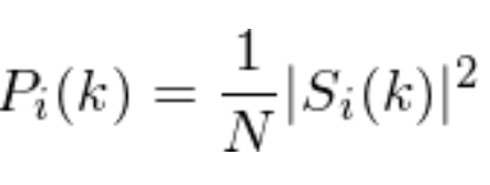
also known as the periodogram estimate of the power spectrum.

You need to take the complex Fourier transform’s absolute value, squaring what you achieve. Broadly speaking we do a 512 point FFT retaining only the first 257 coefficients.

Figure Out the Mel-Spaced Filterbank

It’s a set of 20-40 (26 is the norm) triangle filters.

Going back to the periodic room power spectral estimate in step two, we apply these filters to that.

Continuing with the FFT settings in step two, the filterbank will have 26 vectors of length 257.

Specific sections of the spectrum are non-zero but each vector will mostly be zeros.

We work out filterbank energies by multiplying each filterbank against the power spectrum, summing up the coefficients afterwards.

This should result in 26 numbers that point us towards how much energy is in each filterbank. Head to the section ‘Mel filterbank Computation’ in order to see in detail how filterbanks are calculated.

This figure should help you to understand things:

Make a Log

Next, for the 26 energies from step 3 make a log. You will be left with 26 log filterbank energies.

Discrete Cosine Transform

For those 26 log filterbank, energies make a Discrete Cosine Transform (DCT) to get 26 cepstral coefficients. In the case of ASR, only the bottom 12-13 of the 26 coefficients are retained.

The features we are left with (each frame has 12 numbers) we refer to as Mel Frequency Cepstral Coefficients.

Mel Filterbank Computation

---

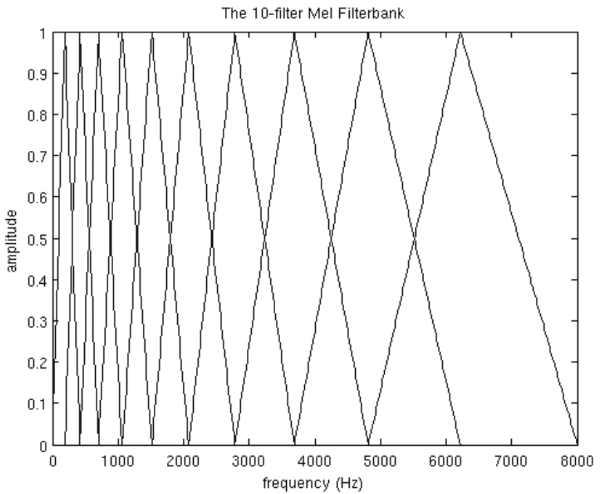
Here we will look at 10 filterbanks for reasons of readability in this tutorial, although 26-40 filterbanks would actually be used.

To produce the filterbanks seen in the diagram and section above you must first select an upper and lower frequency. 8000Hz is good for the upper frequency and 300Hz for the lower.

Keep in mind, if the speech has an 8000 Hz sample then the upper frequency is tapered off to 400Hz maximum.

We then go through the following steps:

Convert the Lower and Upper Frequencies to Mels

Use equation 1 to convert the lower and upper frequencies to Mels. For this example, 8000Hz is 2834.99 Mels and 300Hz is 401.25 Mels. 

Linear Spacing

As said, we’ll use 10 filterbanks for this example, which requires 12 points. This leaves 10 remaining points requiring linear spacing between 401.25 and 2834.99. Which results in:

Revert Back to Hertz

Now use equation 2 to revert back to Hertz:

Do you see how the start and end points are at the expected frequencies?

Rounding the Frequencies

The frequency resolution we have is insufficient to place filters at the specific points shown above, so frequencies need to be rounded to the closest FFT bin.

This doesn’t disturb how accurate the features are. The FFT size and sample rate is needed in order to convert the frequencies to FFT bin numbers:

Which produces this number sequence:

Our last filterbank ends at bin 256, equating to 8kHz with a 512 point FFT size.

Calculating Points

Time to make our filter banks. The first point denotes the beginning of the first filterbank, peaking at the second point, and by the third point reaching back to 0.

The second point denotes the start of the second filter, peaking at the third point, then returning back to 0 at the fourth – and so on. Here’s the formula to calculate this all:

Wherein denotes how many filters we want, and is our list of M+2 Mel–spaced frequencies.

Our last plot of the full 10 filters overlaid atop one another:

Differential and Acceleration Coefficients (Deltas & Delta-Deltas) 

---

A single frame’s power spectral envelope is represented by the MFCC feature vector but nothing more; speech should have more data in the dynamics. In other words, we need to know the MFCC coefficients trajectories over time.

Discerning this and appending the trajectories to the original feature vector improves how well the ASR performs, and by a fair amount.

In the case of 12 MFCC coefficients, we attain a feature vector length of 24, generated by combining 12 delta coefficients.

Let’s run through how to calculate the delta coefficients:

Wherein the delta coefficient is denoted by , from frame calculated based on the static coefficients .

Usually will be the value 2. Acceleration (Delta-Delta) coefficients are discerned through the same process, but using the deltas, not static coefficients.

You Might Also Like:

• Best Cheap VPN
• Best VPN for Android
• Online Privacy Guide
• Turbo VPN Review
• Zenmate VPN