Privacy Canada is community-supported. We may earn a commission when make a purchase through one of our links. Learn more.
Discrete Fourier Transform

This tutorial on discrete Fourier transform (DFT) aims to teach you what that DFT is actually up to.
Many other articles detail the mathematics, but not always in a way that makes it obvious what the mathematics really means.
Several ways exist with which to comprehend the Fourier transform; this tutorial will describe it based on relationships between sinusoids of varying frequencies and a signal.
Discrete Fourier Transform – Intuitive explanation manual
So first an explanation. DFT is an algorithm that accounts for a signal and calculates the ‘frequency content’ of that signal.
In the context of this tutorial, a ‘signal’ is any number sequence, such as the following initial dozen numbers (of a signal that this tutorial will look at in more detail later):
1.00, 0.62, -0.07, -0.87, -1.51, -1.81, -1.70, -1.24, -0.64, -0.15, 0.05, -0.10
The signals are referenced using x(n) wherein n stands for the index into the signal. In this way, x(0) = 1.00, x(2) = -0.07 and so on. You can find signals like this in many circumstances.
For instance, every digital audio signal is made up of number sequences like the above example.
Zero-mean signals will be discussed at the bottom of this tutorial. Zero-mean signals result in a total of 0 when the mean is determined.
By calculating the frequency content, we are in fact trying to simplify a complicated signal into easier portions.
A good number of signals can be best defined as the sum of many separate frequency elements rather than the sum of time-domain samples. DFT is designed to calculate the frequencies that make up a larger more complex signal.
For a more comprehensive account of the DFT consider reading these two text materials:
Digital Signal Processing: Principles, Algorithms and Applications by Proakis and Manolakis – this is the most rigorous account although it needs a fair bit of mathematical experience.
Understanding Digital Signal Processing: by Lyons – if you are new this is a great easy to digest introduction.
DFT Term – ‘Correlation’
Coordination is an often-used idea in signal processing, which you can think of as the quantitative similarity between two separate signals. More correlation means more similarity between signals.
Anything approaching zero means not much similarity. Overall, in the event that you come across this sort of equation:
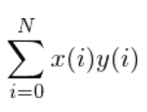
Wherein x and y represent signals, we can think to ourselves “yes!
We are determining how similar x and y are (the correlation!)’ But how does this small equation work out the correlation between two signals?
If y(i) has a strong correlation to x(i), y(i) must be positive if x(i)is positive, and y(i)will normally be negative if x(i)is negative (because the signals are correlated).
Multiplying y(i) and x(i)will always lead to a positive number, whether the numbers were negative or positive, to begin with.
When each of these positive numbers are summed up we are left with a bigger positive number. But what if there is not much correlation? In that event, y(i)may be negative while x(i) is positive or the reverse.
It could also be the case that there is a similarity but both are positive. This is why when we determine the final sum we add some negative numbers and some positive numbers, amounting to something close to 0.
That is a general concept. Signals that result in extreme correlation are very similar, while those that result in low correlation are not, and those that are somewhere in the middle will have a middling correlation score.
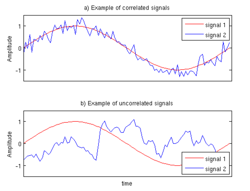
signals examples
I should say at this point that negative correlation is also possible. Any time y(i) is positive and y(i) is negative or the reverse, negative correlation occurs.
This is because any time a positive number is multiplied against a negative number the result is negative.
In the event of a large negative correlation, this also indicates high similarity, just with one signal being the invert of the other.
DFT: The Discrete Fourier Transform
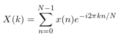
Let’s look at how correlation gives us an insight into the DFT. We’ll start with the DFT equation:
where each DFT coefficient can be determined by sweeping k from 0 to N–1. By “coefficient’ we are talking about X(k), in other words, the value of X(0) equals the value of coefficient 1, X(2) of coefficient 3 and so on.
You should see similarities between this equation and the first correlation equation we discussed in this tutorial because it also determines the correlation between a signal x(n) and a function .
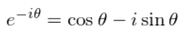
But how should you think about the similarity of a signal with a complex exponential? We can get closer to the heart of the matter by splitting up the exponential into sine and cosine elements with the below identity:
By turning into an updated discrete Fourier transform equation it will look like the following:

And a bit more mathematical logic leads to this:
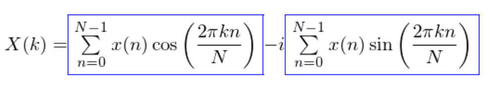
Much simpler! Here we actually have two separate calculations for correlation (each rectangle is indicated by a blue rectangle), one has a cosine wave and the other a sin wave.
Step one is to determine the correlation between a specific frequency of cosine and our signal x(n) and place the achieved value into the real portion of X(k). Next, we repeat the process with a sine wave, placing the achieved value into the imaginary part of X(k).
Investigating Correlation Between a Cosine
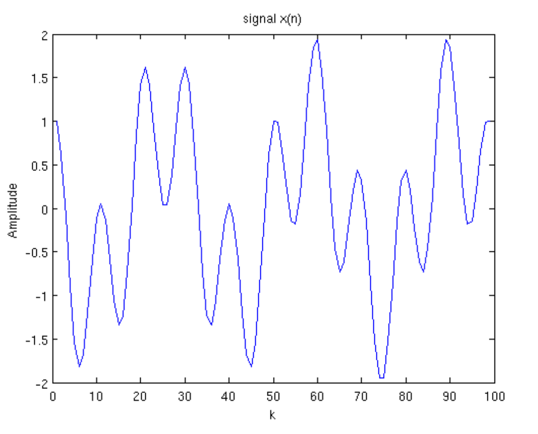
What insights can we glean by looking into the correlation between our signal and a cosine? Let’s take a signal with a 100-long sample length arranged like this:
Let’s run through the process of calculating the correlation level of this signal with a sine and the cosine wave sequence that increases in frequency.
We are going to determine the DFT’s real part through a simulation. Let’s first simulate K=0 with the new equation:
In this example, we determined the signals correlation level with a signal made up only of ones (because cos(0)=1).
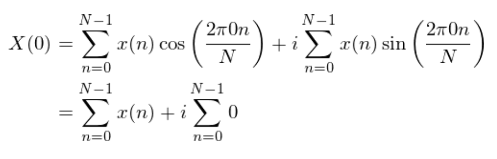
This happens to be the same as the sum of the unaltered signal, which from the example plot should result in about 0 because one half of the signal seems to be above 0 and the other half underneath.
Doing all of the sums the negative elements cancel out the positive elements, which means a correlation of 1.
Setting k = 1 leads to the diagram below: the blue , the red
and black
for plot(a).
for plot(b) and
for plot(c).
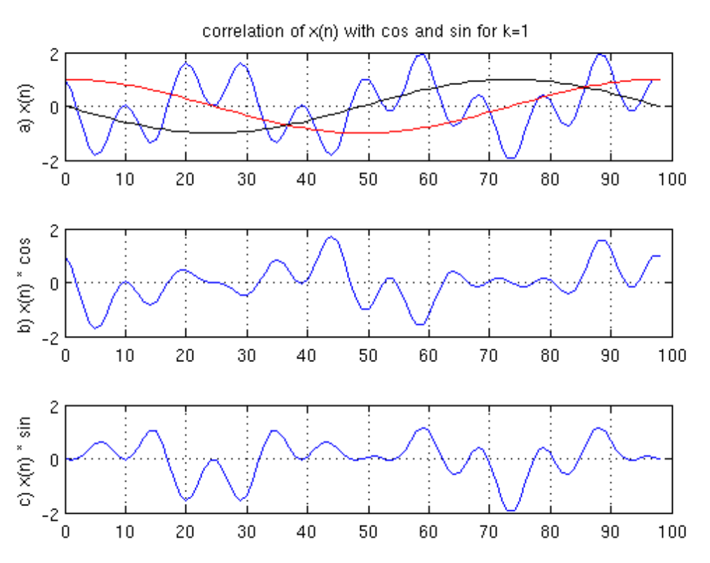
(b) and (c) look to have about half of the signal above zero and a half below, so summing up should produce around zero.
As expected equals one and
equals 0, which means X(1) is 1 + i0.
The next diagram will see the same signals as diagram 3, but with k = 3.
The first plot (a) has cause and sin waves and x(n). The second and third plots show the product of x(n), (b) with the cause signal and (c) with the sin signal.
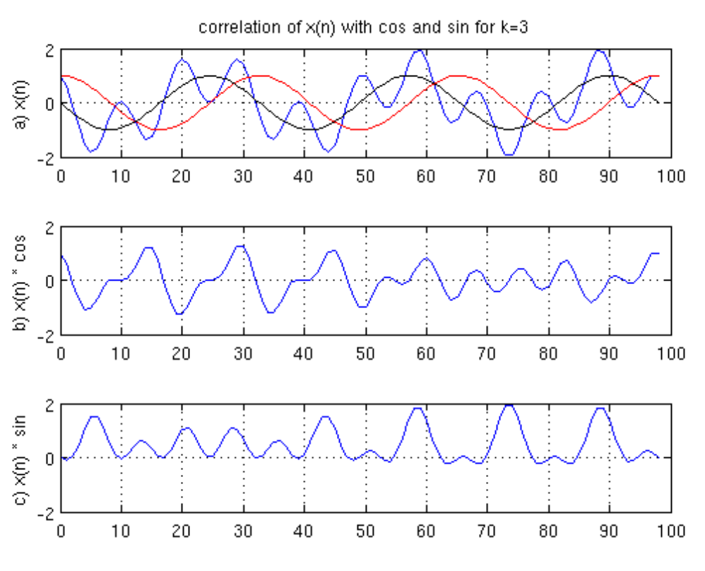
The third plot is nearly fully positive with only a tiny number of negative elements. The cancellation is almost nil resulting in a big positive number.
That also leads to a callsign correlation of 0, with a sin correlation of 49. And the DFT coefficient for k = 3 (X(3)) is 0+i49. You can repeat this process for each K until the full DFT is determined.
Here is how the end DFT looks (on the right is the imaginary part, left is the real part):
As can be seen, k = 10 leads to a real part peak (the signal being similar to a cosine), and for k = 3 there’s the peak in the simulated part (the signal being similar to a sine).
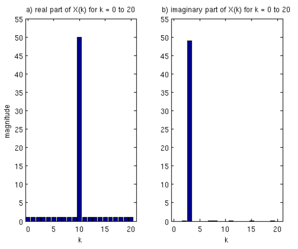
Overall however, it’s unimportant if there is a sine or cosine, we only need to know if a sinusoid is present, regardless of phase.
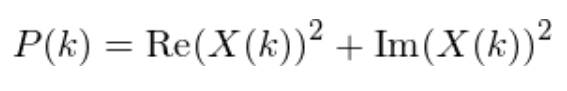
To get this result we integrate the imaginary and real elements to form the power spectrum:
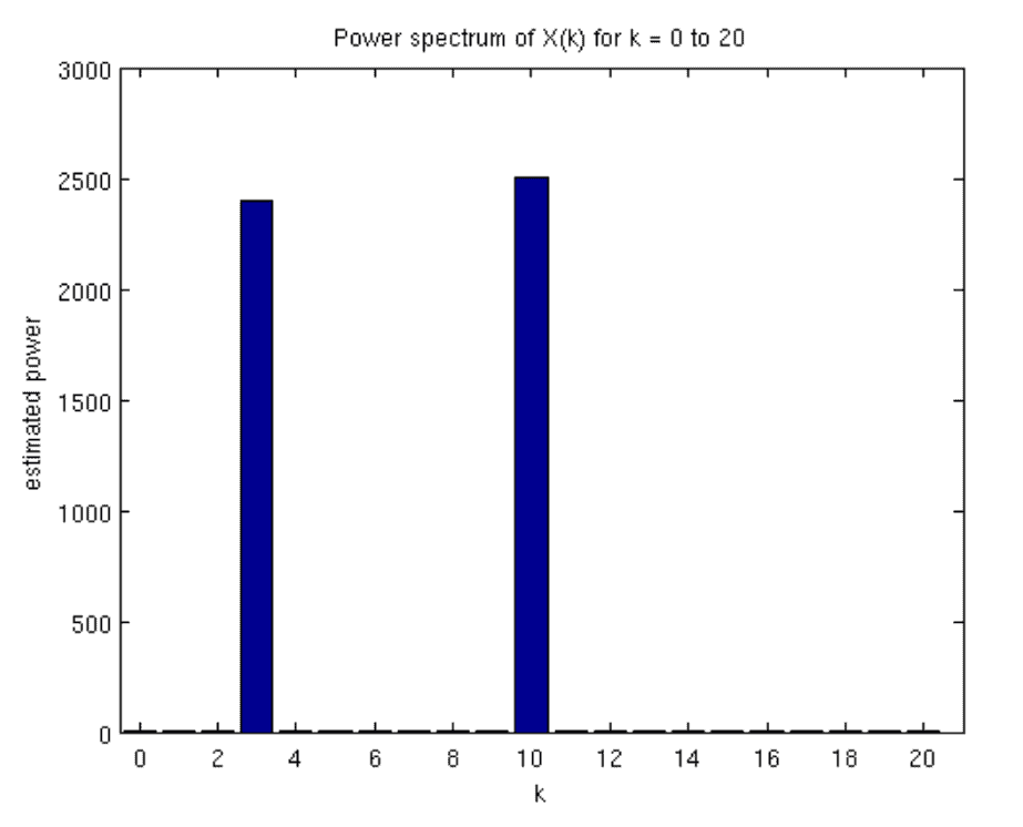
Keep in mind that the power spectrum P(k) has no imaginary element. If we determine the power spectrum from X(k) this results:
The above diagram shows two frequencies in the signal and not much more, which is the thing we wanted to reveal when we began our investigation.
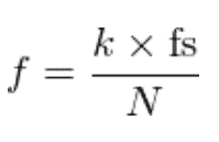
Let’s convert the k values into hertz frequencies, which requires our original signal (fs) sampling rate and this formula:
Wherein fs as our sampling frequency and N how many samples we have in our signal (our above example is 100).
Conclusion
Fun fact that you should know is that discrete Fourier transform is used in Mel frequency Cepstral coefficient which is used in voice recognition systems.
To keep this tutorial simple I have overlooked a few smaller points which I will mention now. I made the assumption that each signal had a zero mean, in which case the similar signals would have a correlation of zero.
This isn’t always the case, but signals are similar whenever correlations are high and dissimilar when lower. Either way, it’s simple enough to subtract the mean when considering signals.
In our example, we determined the DFT for k = 0 to 20. If you continue to determine coefficients for higher k, we would achieve a power spectrum of about N/2.
The real part is an even function for k, while the simulated part odd. To delve deeper into this topic, jump back up to the two books I have recommended in the introduction to this tutorial.